APM_2F005 - Algorithms For Discrete Mathematics Bachelor 2
Lecturer: Lucas Gerin

ToolBox # 1: Graphs and Matrices

## loading python libraries

# necessary to display plots inline:
%matplotlib inline   

# load the libraries
import matplotlib.pyplot as plt # 2D plotting library
import numpy as np              # package for scientific computing  
from math import *              # package for mathematics (pi, arctan, sqrt, factorial ...)

Table of contents

• I. Adjacency matrices and paths in graphs
  • I.1 Definitions
  • I.2 Powers of the adjacency matrix
  • I.3 (Bonus) Application to asymptotics: Perron-Frobenius Theory
• II. Transition matrices and probabilistic graphs
  • II.1 Definitions
  • II.2 Powers of a transition matrix
  • II.3 Absorbing states: experiments and theory
  • II.4 (Bonus) The Markov property

References

Part I: An Introduction to Algebraic Graph Theory. Cesar O. Aguilar. Online Lecture Notes.
Part II: S.M.Ross Introduction to Probability Models (2014), Academic Press.

I. Adjacency matrices and paths in graphs

I.1. Definitions (Review of CSE 102)

Throughout this Notebook a graph $G$ of size $n\geq 1$ is given by $(V,E)$ where:

• $V=\{v_1,\dots,v_n\}$ is a finite set of vertices;
• $E\subset V^2$ is a set of edges.

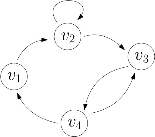
The following is a graphical representation of the graph with

• $V=\{v_1,v_2,v_3,v_4\}$
• $E=\{(v_1,v_2),(v_2,v_2),(v_2,v_3),(v_3,v_4),(v_4,v_4)\}$

Definition. Let $G=(V,E)$ be a graph of size $n$. The adjacency matrix $A_G=(a_{i,j})_{1\leq i,j\leq n}$ associated to $G$ is the $n\times n$ matrix defined by $$ a_{i,j}= \begin{cases} 1 \text{ if the edge }(v_i,v_j)\text{ is in }E ,\\ 0 \text{ otherwise} \end{cases}. $$

In the above example, $$ A_G= \begin{pmatrix} 0 & 1 & 0 & 0\\ 0 & 1 & 1 & 0\\ 0 & 0 & 0 & 1\\ 1 & 0 & 1 & 0\\ \end{pmatrix} $$

I.2. Powers of the adjacency matrix

We will continuously use the following property, as it is the one that makes the introduction of adjacency matrices relevant.

Proposition 1. Let $G=(V,E)$ be a graph of size $n\geq 1$ and $A_G$ be its transition matrix. For $1\leq i,j\leq n$ and $k\geq 1$, denote by $(A_G^k)_{i,j}$ the coefficient $(i,j)$ in $A_G^k$. Then $$ (A_G^k)_{i,j}=\text{Number of paths of length $k$ from $v_i$ to $v_j$ in $G$.} $$

Proof of Proposition 1.
We do the proof in the case $k=2$, the general case follows by induction. Write $A_G=(a_{i,j})_{1\leq i,j\leq n}$. Then by definition of matrix product: $$ (A_G^n)_{i,j}=a_{i,1}a_{1,j}+a_{i,2}a_{2,j}+\dots + a_{i,n}a_{n,j}. $$ Consider a term $a_{i,\ell}a_{\ell,j}$ in the above sum. This term is zero unless $a_{i,\ell}=a_{\ell,j}=1$. The latter means that we have a path of length two $v_i \to v_\ell\to v_j$. In other words $$ a_{i,\ell}a_{\ell,j}= \begin{cases} 1 \text{ if there is a path of length $2$ from $v_i$ to $v_j$, through $v_\ell$} ,\\ 0 \text{ otherwise} \end{cases}. $$ By summing over $\ell$ we obtain the proposition in the case $k=2$.
End of proof.

Numerical application

# Running example

A=np.matrix([[0, 1, 0, 0],
 [0, 1, 1, 0],
 [0, 0, 0, 1],
 [1, 0, 1, 0]]) 

print("A_G:")
print(A)

print('-----')
k=20
print("A_G to the power k =",k,':')
A_to_power_k = A**k
print(A_to_power_k) 

print('-----')
print('There are ',int(A_to_power_k[0,3]), 'paths of length ',k,' from v_1 to v_4')

A_G:
[[0 1 0 0]
 [0 1 1 0]
 [0 0 0 1]
 [1 0 1 0]]
-----
A_G to the power k = 20 :
[[ 529 1024 1208  792]
 [ 792 1553 1816 1208]
 [ 416  792  945  608]
 [ 608 1208 1400  945]]
-----
There are  792 paths of length  20  from v_1 to v_4

I.3. (Bonus) Application to asymptotics: a glimpse of Perron-Frobenius theory.

Let $v_i,v_j$ two vertices of a graph $G$. We want to estimate, for large $k$, the number of paths of length $k$ from $v_i$ to $v_j$. Thanks to Proposition 1 this question amounts to estimating $(A_G^k)_{i,j}$.

In the following proposition we show that the asymptotics is driven by the largest eigenvalue of $A_G$.

Proposition 2 (Simplified version of Perron-Frobenius' Theorem). Let $G=(V,E)$ be a graph of size $n\geq 1$ and $A_G$ be its transition matrix.
Assume that $A_G$ is diagonalizable with $n$ real or complex eigenvalues $\lambda_1,\lambda_2 ,\dots, \lambda_n$. Assume furthermore that for every $2\leq \ell\leq n$ one has $\lambda_1>|\lambda_\ell|$.
Then for every $i,j$ there exists a constant $c_{i,j}\geq 0$ such that, when $k\to+\infty$, $$ \text{Number of paths of length $k$ from $v_i$ to $v_j$ in $G$} = c_{i,j}\lambda_1^k + \mathrm{o}(\lambda_1^k). $$ (In particular this implies that $\lambda_1$ is real.)

Proof of Proposition 2.
We need to estimate the coefficient $(i,j)$ in $A_G^k$. Let us diagonalize $A_G$: $$ A_G=P\times \begin{pmatrix} \lambda_1 & & & &\\ & \lambda_2 & & &\\ & & \lambda_3 & &\\ & & & \ddots & \end{pmatrix} \times Q $$ where $Q=P^{-1}$. Write $P=(p_{i,j})$ and $Q=(q_{i,j})$. (Recall that $(p_{i,\ell})_i$ is an eigenvector for $\lambda_\ell$.) For every $k$ $$ \begin{array}{r c c c c c c} A_G^k&=& P &\times& \begin{pmatrix} \lambda_1^k & & & &\\ & \lambda_2^k & & &\\ & & \lambda_3^k & &\\ & & & \ddots & \end{pmatrix} &\times& Q\\ &=& P &\times& %\begin{matrix} % \\ % \ell\text{-th row}\\ % \\ %\end{matrix} \begin{pmatrix} & & & &\\ & & \lambda_\ell^kq_{\ell,j} & &\\ & & & & \end{pmatrix}_{\ell,j} & & \\ &=& & & \begin{pmatrix} & & & &\\ & & \sum_{\ell}p_{i,\ell}q_{\ell,j}\lambda_\ell^k & &\\ & & & & \end{pmatrix}_{i,j} & & \\ \end{array} $$ Hence \begin{align*} (A_G^k)_{i,j}=\sum_{\ell=1}^np_{i,\ell}q_{\ell,j}\lambda_\ell^k = p_{i,1}q_{1,j}\lambda_1^k+\sum_{\ell=2}^np_{i,\ell}q_{\ell,j}\lambda_\ell^k = p_{i,1}q_{1,j}\lambda_1^k+\mathrm{o}(\lambda_1^k), \end{align*} since $|\lambda_2|,\dots,|\lambda_n|$ are all less than $\lambda_1$. The Proposition is proved, with $c_{i,j}=p_{i,1}q_{1,j}$.
End of Proposition 2.

We want to apply Proposition 2 to our running example. With the following script we compute the eigenvalues of $A$.

# Running example

Diagonalization=np.linalg.eig(A)

Eigenvalues=Diagonalization[0] # Computes the eigenvalues of A
Eigenvectors=Diagonalization[1] # Computes the passage matrix onto the basis of eigenvectors

print('-------')
print('The eigenvalues are:')
print(np.round(Eigenvalues,5))
print('In particular the largest one is')
lambda_1=max(Eigenvalues)
print(np.round(lambda_1,5))
print('-------')
real_parts = Eigenvalues.real
imag_parts = Eigenvalues.imag

# Plots of eigenvalues
plt.figure(figsize=(8, 6))
plt.scatter(real_parts, imag_parts, color='pink', marker='o', s=200) 
plt.axhline(0, color='black',linewidth=0.5)
plt.axvline(0, color='black',linewidth=0.5)
#plt.grid(color = 'gray', linestyle = '--', linewidth = 0.5)
plt.title('Locations of eigenvalues')
plt.xlabel('Real parts')
plt.ylabel('Imaginary parts')
plt.show()

-------
The eigenvalues are:
[-1.17872+0.j       0.33292+0.67077j  0.33292-0.67077j  1.51288+0.j     ]
In particular the largest one is
(1.51288+0j)
-------

We now plot the number of paths of length $k$ from $v_1$ to $v_2$, and compare to $\lambda_1^k$.

def Paths_from_vi_to_vj(i,j,k):
    A_to_power_k = np.linalg.matrix_power(A,k) 
    return A_to_power_k[i-1,j-1]

# We observe that lambda_1 = 1.5128... + 0 \times i where i^2=-1. This is because lambda_1 is obtained
# by numerical approximations. We take the real part in order to avoid this issue.
lambda_1=np.real(lambda_1)

KK=range(40)
NumberOfPaths_v1_v2=[Paths_from_vi_to_vj(1,2,k) for k in KK]
NumberOfPaths_v1_v3=[Paths_from_vi_to_vj(1,3,k) for k in KK]

plt.title('Number of paths')
plt.plot(KK,NumberOfPaths_v1_v2,'o-',label='Paths v_1 to v_2')
plt.plot(KK,NumberOfPaths_v1_v3,'o-',label='Paths v_1 to v_3')
plt.legend()
plt.show()

KK=range(40)
NormalizedNumberOfPaths_v1_v2=[NumberOfPaths_v1_v2[k]/lambda_1**k for k in KK]
NormalizedNumberOfPaths_v1_v3=[NumberOfPaths_v1_v3[k]/lambda_1**k for k in KK]

plt.title('Number of paths divided by lambda_1**k')
plt.plot(KK,NormalizedNumberOfPaths_v1_v2,'o-',label='Paths v_1 to v_2')
plt.plot(KK,NormalizedNumberOfPaths_v1_v3,'o-',label='Paths v_1 to v_3')
plt.legend()
plt.show()

Discussion on the above plots

The plots are consistent with Proposition 2: for instance the number of paths $v_1\to v_2$ seems to be equivalent to $c_{1,2}\lambda_1^k$, where (empirically) $c_{1,2}\approx 0.2600...$ while the number of paths $v_1\to v_3$ seems to be equivalent to $c_{1,3}\lambda_1^k$, with $c_{1,3}\approx 0.3051...$

II. Transition matrices and probabilistic graphs

II.1. Definitions

Definition. Let $G$ be a graph with vertex set $V=\{v_1,\dots,v_n\}$. A transition matrix $P$ over $V$ is a $n\times n$ matrix $P=(p_{i,j})_{1\leq i,j\leq n}$ such that:

• each coefficient $p_{i,j}$ is in $[0,1]$;
• for all $1\leq i\leq n$, one has $\sum_{j=1}^n p_{i,j}=1$.

Here is an example of a transition matrix over some set $\{v_1,\dots,v_4\}$: $$ P= \begin{matrix} v_1 \\ v_2 \\ v_3\\ v_4 \end{matrix} \begin{pmatrix} 1/4 & 1/4 & 1/2 & 0\\ 1/2 & 0 & 1/4 & 1/4\\ 0 & 0 & 1 & 0\\ 0 & 0 & 0 & 1\\ \end{pmatrix} $$ It is often convenient to represent a transition matrix as a probabilistic graph: we put an edge $v_i\to v_j$ with a weight $p_{i,j}$. The above matrix $P$ corresponds to the following probabilistic graph:

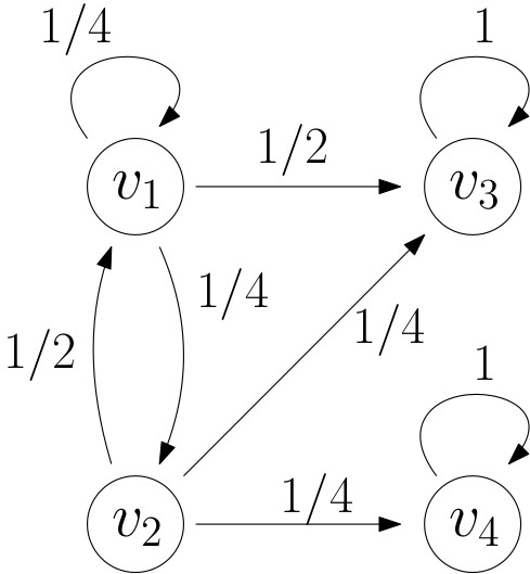
A transition matrix is used to model the random process of an individual (which may be a particle in a physical system, an agent in a model in economics, an internal variable in a stochastic algorithm, ...) on the set $V$. The coefficient $p_{i,j}$ is interpreted as the probability of going from $v_i$ to $v_j$ in exactly one time step.
The good framework for such a model is that of Markov chains.

Definition. Let $P$ be a transition matrix over some vertex set $V$, and let $v_{i_0}\in V$ be a particular vertex called starting point.
A Markov chain $(X_t)_{t\in \mathbb{N}}$ with transition matrix $P$ and starting point $v_{i_0}$ is a sequence of random variables such that

• $X_0=v_{i_0}$;
• For every $t\geq 1$, every $t$-uple $v_{i_1},\dots v_{i_t}$ of vertices, $$ \mathbb{P}\left(X_1=v_{i_1},\dots,X_t=v_{i_t}\right) = p_{i_0,i_1}\times p_{i_1,i_2}\times \dots\times p_{i_{t-1},i_t}. $$

II.2. Powers of a transition matrix

Successive powers of a transition matrix $P$ allow to compute the distribution of a Markov chain at a given time.

Proposition 3. Let $(X_t)_{t\in \mathbb{N}}$ be a Markov chain of transition matrix $P$ over some vertex set $\{v_1,\dots,v_n\}$. Denote by $v_{i_0}$ its starting point.
Then for every $t\geq 1$ and every vertex $v_j$, $$ \mathbb{P}(X_t=v_j) = (P^t)_{i_0,j}. $$

Proof of Proposition 3.
By the law of total probabilities \begin{align*} \mathbb{P}(X_{t}=v_{i_{j}}) &= \sum_{i_1,\dots,i_{t-1}\in V}\mathbb{P}\left( X_1=v_{i_1},\dots,X_{t-1}=v_{i_{t-1}},X_{t}=v_{i_{j}}\right)\\ &= \sum_{i_1,\dots,i_{t-1}\in V}p_{i_0,i_1}\times p_{i_1,i_2}\times \dots \times p_{i_{t-2},i_{t-1}}\times p_{i_{t-1},j}\\ &= (P^t)_{i_0,j}. \end{align*} (If the last equality is not clear to you, you can try to prove it by induction on $t$.)

End of Proposition 3.

Application to our example:

P=np.matrix([
[1/4, 1/4, 1/2, 0],
[1/2, 0  , 1/4, 1/4],
[0,0,1,0],
[0,0,0,1],
]) 
print('-----')
print("P =")
print(P)

print('-----')
t=6
print("P to the power ",t)
P_to_power_t = np.linalg.matrix_power(P,t) # computes P**t
print(np.round(P_to_power_t,4)) 
print('-----')
print('Asumme X_0=v_1. At time t =',t,' X_t is at position v_2 with probability ',np.round(P_to_power_t[0,1],4))

-----
P =
[[0.25 0.25 0.5  0.  ]
 [0.5  0.   0.25 0.25]
 [0.   0.   1.   0.  ]
 [0.   0.   0.   1.  ]]
-----
P to the power  6
[[0.0105 0.0051 0.887  0.0974]
 [0.0103 0.0054 0.687  0.2974]
 [0.     0.     1.     0.    ]
 [0.     0.     0.     1.    ]]
-----
Asumme X_0=v_1. At time t = 6  X_t is at position v_2 with probability  0.0051

II.3. Absorbing states: experiments and theory.

A look at the probabilitic graph of our previous example shows that if the particle hits $v_3$ it stays at $v_3$ forever (the same happens at $v_4$). We say that $v_3$ and $v_4$ are absorbing states for the chain $(X_t)$.

The following question is natural: what is the probability that, starting from $v_1$, the chain is absorbed at $v_3$? at $v_4$?

If we compute $P^t$ for a large $t$ in our example, we obtain:

print('-----')
t=30
print("P to the power ",t)
P_to_power_t = np.linalg.matrix_power(P,t) # computes A**t
print(np.round(P_to_power_t,4)) 
print('-----')
for starting_point in [0,1]:
    for absorbing_state in [2,3]:
        print('Asumme X_0=v_'+str(starting_point+1)+'. At time t ='+str(t)+' X_t is at position v_'+str(absorbing_state+1)+' with probability '+str(np.round(P_to_power_t[starting_point,absorbing_state],10)))

-----
P to the power  30
[[0.  0.  0.9 0.1]
 [0.  0.  0.7 0.3]
 [0.  0.  1.  0. ]
 [0.  0.  0.  1. ]]
-----
Asumme X_0=v_1. At time t =30 X_t is at position v_3 with probability 0.8999999992
Asumme X_0=v_1. At time t =30 X_t is at position v_4 with probability 0.0999999998
Asumme X_0=v_2. At time t =30 X_t is at position v_3 with probability 0.6999999992
Asumme X_0=v_2. At time t =30 X_t is at position v_4 with probability 0.2999999998

This suggests that if the starting point is $v_1$ then $$ \mathbb{P}(\text{the chain is absorbed at }v_3)\approx 0.9,\qquad \mathbb{P}(\text{the chain is absorbed at }v_4)\approx 0.1. $$ In this Section we do not state a general result but rather explain on this example how to compute exactly the absorbing probabilities.

For an arbitrary state $v_i$ and an absorbing state $a$, let $\alpha_{v_i}^{a}$ be the probability that, starting at $v_i$, the chain is absorbed at $a$. Of course $$ \alpha_{v_3}^{v_3}=\alpha_{v_4}^{v_4}=1,\qquad \alpha_{v_3}^{v_4}=\alpha_{v_4}^{v_3}=0. $$ We write \begin{align*} \alpha_{v_1}^{v_3}&=\mathbb{P}(X_0=v_1,\text{the chain is absorbed at }v_3)\\ &=\mathbb{P}(X_0=v_1,X_1=v_1,\text{the chain is absorbed at }v_3)+ \mathbb{P}(X_0=v_1,X_1=v_2,\text{the chain is absorbed at }v_3)+ \mathbb{P}(X_0=v_1,X_1=v_3,\text{the chain is absorbed at }v_3)\\ &= p_{1,1}\alpha_{v_1}^{v_3}+p_{1,2}\alpha_{v_2}^{v_3}+p_{1,3}\alpha_{v_3}^{v_3}\\ &= \frac{1}{4}\times \alpha_{v_1}^{v_3}+\frac{1}{4}\alpha_{v_2}^{v_3}+\frac{1}{2}. \end{align*} If we do the same starting from $v_2$ we get \begin{align*} \alpha_{v_2}^{v_3}&= \frac{1}{2}\times \alpha_{v_1}^{v_3}+\frac{1}{4}+\frac{1}{4}\times 0. \end{align*} Finally we have the $2\times 2$ linear system $$ \begin{cases} \alpha_{v_1}^{v_3}&=\frac{1}{4}\times \alpha_{v_1}^{v_3}+\frac{1}{4}\alpha_{v_2}^{v_3}+\frac{1}{2}\\ \alpha_{v_2}^{v_3}&= \frac{1}{2}\times \alpha_{v_1}^{v_3}+\frac{1}{4} \end{cases} \Leftrightarrow \begin{cases} \alpha_{v_1}^{v_3}&=9/10\\ \alpha_{v_2}^{v_3}&=7/10 \end{cases}, $$ which is consistent with our numerical approximation.

II.4. Bonus: The Markov property

The following property is fundamental for Markov chains. It tells that in order to compute the distribution of $X_{t+1}$, it is enough to know the distribution of $X_t$.

Proposition 3 (Markov Property). Let $(X_t)_{t\in \mathbb{N}}$ be a Markov chain with transition matrix $P$. For every $t\geq 1$, and every $t+1$-uple $v_{i_1},\dots v_{i_{t+1}}$ of vertices, $$ \mathbb{P}\left(X_{t+1}=v_{i_{t+1}}\ |\ X_1=v_{i_1},\dots,X_t=v_{i_t}\right) = \mathbb{P}\left(X_{t+1}=v_{i_{t+1}}\ |\ X_t=v_{i_t}\right) =p_{i_t,i_{t+1}}. $$

Proof of Proposition 3.
We first compute the left-hand side, using the definition of conditional probabilities: \begin{align*} \mathbb{P}\left(X_{t+1}=v_{i_{t+1}}\ |\ X_1=v_{i_1},\dots,X_t=v_{i_t}\right) &= \frac{\mathbb{P}\left( X_1=v_{i_1},\dots,X_t=v_{i_t},X_{t+1}=v_{i_{t+1}}\right)}{\mathbb{P}\left( X_1=v_{i_1},\dots,X_t=v_{i_t}\right)}\\ &= \frac{p_{i_0,i_1}\times p_{i_1,i_2}\times \dots p_{i_{t-1},i_t}\times p_{i_{t},i_{t+1}}}{p_{i_0,i_1}\times p_{i_1,i_2}\times \dots\times p_{i_{t-1},i_t}}\\ &= p_{i_{t},i_{t+1}}. \end{align*} Let us now compute the right-hand side, using the law of total probabilities: \begin{align*} \mathbb{P}\left(X_{t+1}=v_{i_{t+1}}\ |\ X_t=v_{i_t}\right) &= \frac{\mathbb{P}\left( X_t=v_{i_t},X_{t+1}=v_{i_{t+1}}\right)}{\mathbb{P}\left(X_t=v_{i_t}\right)}\\ &= \frac{\sum_{i_0,\dots,i_{t-1}\in V}\mathbb{P}\left( X_1=v_{i_1},\dots,X_t=v_{i_t},X_{t+1}=v_{i_{t+1}}\right)}{\sum_{i_0,\dots,i_{t-1}\in V}\mathbb{P}\left( X_1=v_{i_1},\dots,X_t=v_{i_t}\right)}\\ &= \frac{\sum_{i_0,\dots,i_{t-1}\in V}p_{i_0,i_1}\times p_{i_1,i_2}\times \dots p_{i_{t-1},i_t}\times p_{i_{t},i_{t+1}}}{\sum_{i_0,\dots,i_{t-1}\in V}p_{i_0,i_1}\times p_{i_1,i_2}\times \dots\times p_{i_{t-1},i_t}}\\ &= \frac{p_{i_{t},i_{t+1}}\sum_{i_0,\dots,i_{t-1}\in V}p_{i_0,i_1}\times p_{i_1,i_2}\times \dots p_{i_{t-1},i_t}}{\sum_{i_0,\dots,i_{t-1}\in V}p_{i_0,i_1}\times p_{i_1,i_2}\times \dots\times p_{i_{t-1},i_t}}\\ &= p_{i_{t},i_{t+1}}. \end{align*} End of proof of Proposition 3.