APM_2F005 - Algorithms For Discrete Mathematics Bachelor 2
Lecturer: Lucas Gerin

Graphs and Matrices 1: Adjacency Matrices

Table of contents

• 1. Adjacency Matrices
• 2. Enumeration of words
• 3. Transition Matrices and Absorption probabilities
• Bonus. The target

## loading python libraries

# necessary to display plots inline:
%matplotlib inline   

# load the libraries
import matplotlib.pyplot as plt # 2D plotting library
import numpy as np              # package for scientific computing  

from math import *              # package for mathematics (pi, arctan, sqrt, factorial ...)

1. Adjacency Matrices

Exercise 1. Warm-up

Let $G$ be the following graph:

Use the adjacency matrix of $G$ to compute the number of paths of length $20$ from $d$ to $c$ in $G$.

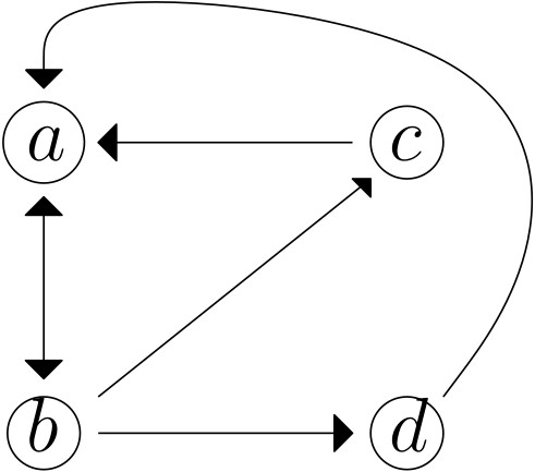
AdjacencyMatrix=np.matrix([[0,1,0,0],[1,0,1,1],[1,0,0,0],[1,0,0,0]])
n=20
B=AdjacencyMatrix**n
print(str(B[3,3])+' paths of length '+str(n))

#print(B)

488 paths of length 20

The number of paths is given by the coefficient corresponding to $(d,c)$ (i.e. coeff.$(4,3)$) in $A^{20}$, where $A$ is given by $$ A= \begin{matrix} a \\ b \\ c\\ d \end{matrix} \begin{pmatrix} 0 & 1 & 0 & 0\\ 1 & 0 & 1 & 1\\ 1 & 0 & 0 & 0\\ 1 & 0 & 0 & 0 \end{pmatrix}. $$

2. Enumeration of words

Exercise 2. $b$ never followed by $c$

We consider words with letters $a,b,c$. Let $M_n$ be the number of words of length $n$ (the length of a word is the number of letters) such that a $b$ is never immediately followed by a $c$. For example $M_2=8$: $$ aa,\ ab,\ ac,\ ba,\ bb,\ ca,\ cb,\ cc. $$ Question 1. Write a script which computes $M_1,M_2,\dots,M_{20}$ using a graph and its adjacency matrix. You can consider the following graph:

Question 1. The number $S_n$ corresponds to the number of paths of length $n-1$ in the above graph ($n-1$ edges correspond to $n$ letters.) For exemple, the word $abbbac$ (length $6$) corresponds to $a\to b\to b\to b\to a\to c$ (path of length $5$). Therefore $M_n$ is the sum of all coefficients in the matrix $A^{n-1}$, where $$ A= \begin{matrix} a \\ b \\ c \end{matrix} \begin{pmatrix} 1 & 1 & 1 \\ 1 & 1 & 0 \\ 1 & 1 & 1 \\ \end{pmatrix}. $$

# Matrices of b-short words
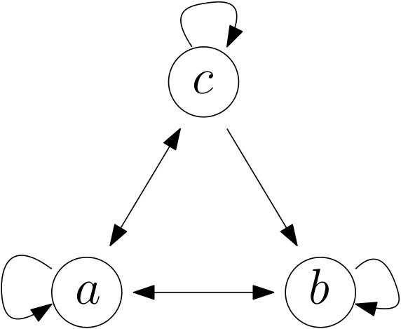
Adjacency_abc=np.matrix([[1,1,1],[1,1,0],[1,1,1]])
#print('Adjacency matrix : ')
#print(Adjacency_abc)
List=[]
for n in range(1,21):
    Mat=Adjacency_abc**(n-1)
    List.append(np.sum(Mat))
    print('Number of words of size n=',n,': ',np.sum(Mat))

Exercise 3. $b$-short words

We say that a word $w$ with letters $a,b$ is $b$-short if there are never $4$ consecutive $b$'s in $w$. For instance, $$ w_1=aa\color{green}{b}aaaaaa\color{green}{bbb}aaa\color{green}{b}aa $$ is $b$-short while $$ w_2=aa\color{green}{b}aa\color{green}{bb}a\color{red}{bbbbbb}aa\color{green}{bb}a $$ is not. Let $S_n$ be the number of $b$-short words of length $n$. Write a script which computes $S_1,S_2,\dots,S_{20}$ using a graph and its adjacency matrix.

Question 1. The number $S_n$ corresponds to the number of paths starting from $a$ or $b$ and of length $n-1$ in the graph whose adjacency matrix is $$ A= \begin{matrix} a \\ b \\ b' \\ b'' \end{matrix} \begin{pmatrix} 1 & 1 & 0 & 0\\ 1 & 0 & 1 & 0\\ 1 & 0 & 0 & 1\\ 1 & 0 & 0 & 0 \end{pmatrix}. $$ For exemple, the word $abbbaa$ (length $6$) corresponds to $a\to b\to b'\to b''\to a\to a$ (path of length $5$).
(The vertices $b,b',b''$ ensure that there are never $4$ consecutive $b$'s.) Therefore $S_n$ is the sum of all coefficients in the two first rows of matrix $A^{n-1}$. (If we take the sum of all coefficients, we will count three times some words beginning with $b$.)

# Matrices of b-short words
Adjacency_bShort=np.matrix([[1,1,0,0],[1,0,1,0],[1,0,0,1],[1,0,0,0]])
#print('Adjacency matrix : ')
#print(Adjacency_bShort)

for n in range(1,21):
    Mat=Adjacency_bShort**(n-1)
    MatBis=Mat[0:2,]
    print('For n = ',n,' there are ', np.sum(MatBis),' b-short words')

3. Transition matrices

Exercise 4. Labyrinth.

We consider a random robot in the following labyrinth:

The robot is initially in room $B$ (time $n=0$). At each time step, it chooses uniformly at random one of the doors of the room in which it is located, and passes through that door.
If the robot hits Exit $1$ (resp. $2$) it stays at Exit $1$ (resp. $2$) forever.

Let $p(n)$ denote the vector of the probability distribution of the location of the robot at time $n$. More formally, $$ p(n)=\bigg(p_x(n) \bigg)_{x\in \{A,B,C,D,E,\text{Exit }1,\text{Exit }2\}}, $$ where $p_x(n)$ is the probability that the robot is at $x$ at time $n$. Of course we have that $$ p(0)=(0,1,0,0,0,0,0). $$ 1) Use a transition matrix $M$ to compute approximate values of $p(5)$ and $ p(100)$. 2) If we wait long enough the robot eventually escapes the labyrinth, either through Exit 1 or Exit 2. By raising $M$ to some large enough power ($100$ should be fine), find a numerical approximation of the probability that the robot escapes the labyrinth through Exit $1$.

1. We consider the following transition matrix: $$ M= \begin{matrix} A \\ B \\ C \\ D \\ E \\ E1 \\ E2 \end{matrix} \begin{pmatrix} 0 & 1/2 & 0 & 1/2 & 0 & 0 & 0\\ 1/3 & 0 & 1/3 & 0 & 1/3 & 0 & 0\\ 0 & 1/2 & 0 & 0 & 0 & 1/2 & 0\\ 1/2 & 0 & 0 & 0 & 1/2 & 0 & 0\\ 0 & 1/3 & 0 & 1/3 & 0 & 0 & 1/3\\ 0 & 0 & 0 & 0 & 0 & 1 & 0\\ 0 & 0 & 0 & 0 & 0 & 0 & 1 \end{pmatrix}. $$ We have seen in the Lecture that the coefficient $(i,j)$ in $M^{n}$ corresponds to the probability that, starting from $i$-th state, the robot is at $j$ at time $n$. Therefore the desired probability distribution is the $2$d line of $M^{n}$.

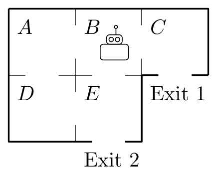
A=np.matrix([
[0,0.5,0,0.5,0,0,0],
[1/3.0,0,1/3.0,0,1/3.0,0,0],
[0,0.5,0,0,0,0.5,0],
[1/2.0,0,0,0,1/2.0,0,0],
[0,1/3.0,0,1/3.0,0,0,1/3.0],
[0,0,0,0,0,1,0],
[0,0,0,0,0,0,1],    
])
#print(np.round(A**80,3))

def ProbaDistribution(n):
    Power=np.linalg.matrix_power(A,n)
    return Power[1,:]

print('------- Question 1 -----')
print('Approximation of probability distributions:')
for n in [5,100]:
    print('p(',n,') = ',str(np.round(ProbaDistribution(n),3)))

print('------- Question 2 -----')

for n in [100]:
    Distribution=ProbaDistribution(n)
    print('At time n=',n,', the robot is at Exit 1 with probab. '+str(np.round(Distribution[0,5],6)))
    

2) For $n=100$ we have that the robot is at Exit $1$ with probability $\approx 0.467$ and at Exit $2$ with probability $0.533$. We see that other coefficients are very close to zero so it is very unlikely that the robot is still in the labyrinth at time $100$. Therefore our approximation is $0.467$.

We still assume that the robot starts at $B$.
Denote by $L_n$ the event "The robot is still in the labyrinth at time $n$" (i.e. it dit not find the exit yet).
1) Use your matrix $M$ to plot $n\mapsto \mathbb{P}(L_n)$. (Try $1\leq n\leq 40$.)

def ProbaNoEscape(n):
    Distribution=ProbaDistribution(n)
    return 1-Distribution[0,5]-Distribution[0,6] # returns 1-Proba(Exit 1)-Proba(Exit 2)

N=30

Proba=[ProbaNoEscape(n) for n in range(N)]

plt.plot(Proba,'o-')
plt.show()

Question 3). For $x\in \{A,B,C,D,E\}$ let $\pi_x$ be the probability that starting from $x$ the robot exits the labyrinth through Exit 1.
Write a system of equations for $\pi_A, ...,\pi_E$ (you can use the method explained in the Math Toolbox). Use `numpy` to solve the system and compare with your approximation obtained previously.
NB: If you want to solve with `numpy` the system $$ \begin{cases} x+3y&=1\\ 2x-y&=0 \end{cases} $$ you can use `np.linalg.solve`: ``` A=np.array([[1,3],[2,-1]]) B=np.array([1,0]) print(np.linalg.solve(A, B)) ```

Let $(X_n)$ be the location of the robot at time $n$, according the method seen in class, we condition on $X_1$: \begin{align*} \pi_A&=\mathbb{P}\left( (X_n) \text{ is eventually absorbed at Exit 1}\ | X_0=A \right)\\ &=\mathbb{P}\left( (X_n) \text{ is eventually absorbed at Exit 1}, X_1=B\ | X_0=A \right)\\ & + \mathbb{P}\left( (X_n) \text{ is eventually absorbed at Exit 1}, X_1=D\ | X_0=A \right)\\ &=\pi_B\mathbb{P}(X_1=B\ | X_0=A)+\pi_D\mathbb{P}(X_1=D\ | X_0=A)\\ &=\pi_B\times 1/2+\pi_D\times 1/2. \end{align*} Other equations are proved similarly: $$ \begin{cases} \pi_A&=\frac{1}{2}\pi_B+\frac{1}{2}\pi_D\\ \pi_B&=\frac{1}{3}\pi_A+\frac{1}{3}\pi_C+\frac{1}{3}\pi_E\\ \pi_C&=\frac{1}{2}\pi_B+\frac{1}{2}\\ \pi_D&=\frac{1}{2}\pi_A+\frac{1}{2}\pi_E\\ \pi_E&=\frac{1}{3}\pi_B+\frac{1}{3}\pi_D\\ \end{cases} $$ We solve this system with the code below and obtain indeed $$ \pi_B\approx 0.4666... $$

A=np.array([[1,-1/2,0,-1/2,0],
            [-1/3,1,-1/3,0,-1/3],
            [0,-1/2,1,0,0],
            [-1/2,0,0,1,-1/2],
            [0,-1/3,0,-1/3,1]])
B=np.array([0,0,1/2,0,0])
print(np.linalg.solve(A, B))

Bonus: The target

A player plays the following game:

• A target $T \in \{1,2,3,\dots \}$ is fixed.
• The player starts from $0$ and keeps throwing a fair die (with six faces) until the cumulative sum is $\geq T$ and then stops.
• If the player ends right on $T$ then the player has won, otherwise (i.e. the player ends on $T+1$, $T+2$,..., $T+5$) the player has lost.

Here is an example with $T=12$: $$ 0 \stackrel{\text{dice = }3}{\longrightarrow} 3 \stackrel{\text{dice = }5}{\longrightarrow} 8\stackrel{\text{dice = }1}{\longrightarrow} 9\stackrel{\text{dice = }4}{\longrightarrow} 13\ \text{(Lost)} $$

Write a function or a script in python which computes the winning probability $p_T$ when the target is $T$. Explain your strategy and justify that it is correct.

In order to check your code: $$ p_1=0.166667\dots,\quad p_2=0.194444\dots,\quad p_9=0.280369\dots $$

We consider a Markov chain on the set $\{0,1,2,\dots , T,T+1,\dots T+5 \}$ which represents the successive cumulative sums of dice. (Once it reaches $T$ or more the process is over.) The corresponding transition matrix is then $$ M= \begin{matrix} 0 \\ 1 \\ 2 \\ \vdots \\ T-1 \\ T \\ T+1 \\ \vdots \\ T+5 \end{matrix} \begin{pmatrix} 0 & 1/6 & 1/6 & \dots & 1/6 & 0 & 0& \dots & 0 & 0 & 0 & 0 \\ 0 & 0 & 1/6 & \dots & 1/6 & 1/6 & 0 & \dots & 0 & 0 & 0 & 0 \\ & & & \ddots & & & & & & & \\ & & & & & & & & & & &\\ & & & & & & & & 1/6 & \dots & 1/6 & 1/6 \\ & & & & & & & & 1 & & &\\ & & & & & & & & & 1 & &\\ & & & & & & & & & & 1 &\\ & & & & & & & & & & &1 \\ \end{pmatrix}. $$ The process is over (in the worst case) at time $T$ since at every step the cumulative sum increases by as least $1$. At time $T$, the chain as thus reached one of the absorbing states $\{T,T+1,\dots,T+5\}$. So the winning probability is $$ \mathbb{P}(\text{The process hits }T)=(M^T)_{0,T}. $$

T=9 # target

# We consider a transition matrix 
Matrix_target=np.zeros([T+6,T+6])
for i in range(T):
    for j in range(i+1,i+7):
        Matrix_target[i,j]=1/6
for l in range(T,T+6):
    Matrix_target[l,l]=1
        
#print(np.round(Matrix_target,2))

# Transition matrix raised to the power T:
Power=np.linalg.matrix_power(Matrix_target,T)

# Test: should return 0.2803689
print('Test: should be equal to 0.2803689:')
print(Power[0,T])

For which target $1\leq T \leq 30$ is the game the most favourable?

n=30
XX=range(1,n+1)
plt.plot(XX,[WinningProbability(n,6) for n in XX],'o-')
plt.show()

According to the above plot the game is the most favourable for $T=6$.

(In passing we observe that $(p_T)_T$ seems to converge. Indeed it can be proved using Markov chains that $$ \lim_T p_T=\frac{1}{7/2}=0.2857... $$ The intuition is that the average dice outcome is $7/2$ so that a large $T$ has approximately a probability $\frac{1}{7/2}$ of belonging to $\mathrm{Cumul}$.)