APM_2F005 - Algorithms For Discrete Mathematics Bachelor 2
Lecturer: Lucas Gerin

Graphs and Matrices 2: Solving some Probabilistic Models

Table of contents

• Model 1: The Frog
• Model 2: Opinion propagation among sheep
• Model 3: OK Corral
• Bonus: The birthday paradox

## loading python libraries

# necessary to display plots inline:
%matplotlib inline   

# load the libraries
import matplotlib.pyplot as plt # 2D plotting library
import numpy as np              # package for scientific computing  

from math import *              # package for mathematics (pi, arctan, sqrt, factorial ...)
import sympy as sympy             # package for symbolic computation
from sympy import *

Model 1: The frog (or how to become a trader?)

This is a math puzzle that used to be asked in job interviews for positions such as quantitative analysts or traders.

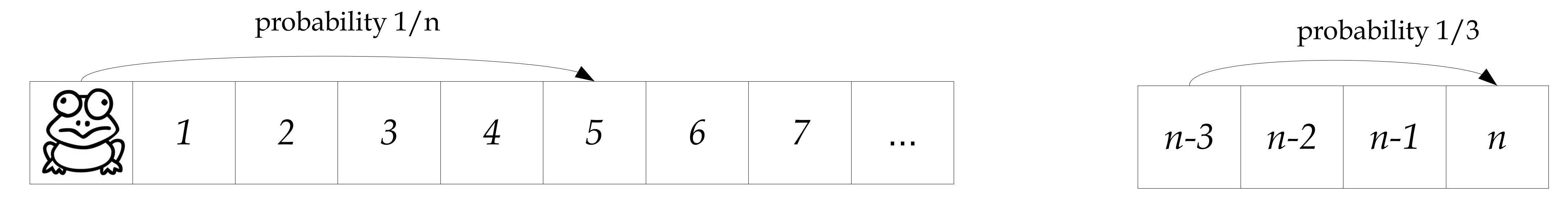
Here is the puzzle: a frog starts at the bank of a river located at $x=0$. The opposite bank is at $x=10$. The frog's first jump is chosen uniformly at random from ${1, 2, \dots, 10}$ (if it lands on $10$, the frog crosses the river and the process ends). Afterward, at each time step, if the frog is at some position $y<10$, it jumps to a uniform random location in ${y+1, \dots, 10}$.

The question is: what is the probability distribution of the total number of steps needed for the frog to cross the river?
(During the job interview, candidates were given access to a computer with a programming language.)

For $n\geq 0$ let $X_n\in\{0,1,\dots, 10\}$ be the location of the frog at time $n$. Let also $T$ be the random variable given by the number of steps needed to reach the other bank. Namely, $$ T=\min \{n\geq 0\text{ such that }X_n=10\}. $$ 1. Write a script which computes the transition matrix $Q=(Q_{i,j})_{0\leq i,j \leq 10} $ associated to the Markov chain $(X_n)_n$. 2. Write a function `DistributionFrog(i,n)` which computes the probability that the frog is at location `i` at time `n` (i.e. $\mathbb{P}(X_n=i)$). 3. For any $1\leq t\leq 10$ write $\mathbb{P}(T\leq t)$ under the form $\mathbb{P}(X_n=i)$ for some well chosen $n$ and $i$. Deduce how to compute $\mathbb{P}(T= t)$ using the transition matrix $Q$. 4. Plot the distribution $t\mapsto \mathbb{P}(T=t)$. What is the most probable value for $T$?

1. Let $L=10$. Starting from a given $i$ the frog jumps at $i< j\leq L$ with probability $1/(L-i)$. Therefore for $ii},\\ 0 & \text{ otherwise.} \end{cases} $$ If $i=L$ then we take the convention that the frog stays still at $L$: $Q_{L,L}=1$. 2. By the course formula we have $\mathbb{P}(X_n=i)=(Q^n)_{0,i}$. 3. We first observe that the event $\{X_t=10\}$ exactly means that the frog has reached the bank at time $t$ or before: $\{X_t=10\}=\{T\leq t\}$. Therefore \begin{align*} \mathbb{P}(T=t)&=\mathbb{P}(T\leq t)-\mathbb{P}(T\leq t-1)\\ &=\mathbb{P}(X_t=10)-\mathbb{P}(X_{t-1}=10)\\ &= (Q^t)_{0,10}-(Q^{t-1})_{0,10}. \end{align*}

# Question 1
def MatrixFrog(L):
    # L = length of the river (L=10 in the exercise)
    # returns the transition matrix of the location of the frog
    Matrix=np.zeros([L+1,L+1])
    Matrix[L,L]=1 # absorbing state
    for i in range(L):
        for j in range(i+1,L+1):
            Matrix[i,j]=1/(L-i)  
    return Matrix

print('---- Question 1 ---')
print('The transition matrix Q = ')
print(np.round(MatrixFrog(6),3))

# Question 2
def DistributionFrog(L,i,t):
    # L = length of the river (L=10 in the exercise)
    # 0 <= i <= L : location of the frog
    # t : time step
    Power_of_M=np.linalg.matrix_power(MatrixFrog(L),t)
    return Power_of_M[0,i]
    
print('---- Question 2 ---')
t=3    
print('Distribution of X at time t =',t,' is ',[np.round(DistributionFrog(10,i,t),2) for i in range(11)])

# Question 3

def DistributionT(L,t):
    if t==0:
        return 0
    return DistributionFrog(L,L,t)-DistributionFrog(L,L,t-1)

print('---- Question 3 ---')

L=10
plt.plot(range(1,L+1),[DistributionT(L,t) for t in range(1,L+1)],'o-',label='t -> P(T=t)')
plt.title('Distribution of T')
plt.xticks(range(1,L+1))
plt.legend()
plt.show()

---- Question 1 ---
The transition matrix Q = 
[[0.    0.167 0.167 0.167 0.167 0.167 0.167]
 [0.    0.    0.2   0.2   0.2   0.2   0.2  ]
 [0.    0.    0.    0.25  0.25  0.25  0.25 ]
 [0.    0.    0.    0.    0.333 0.333 0.333]
 [0.    0.    0.    0.    0.    0.5   0.5  ]
 [0.    0.    0.    0.    0.    0.    1.   ]
 [0.    0.    0.    0.    0.    0.    1.   ]]
---- Question 2 ---
Distribution of X at time t = 3  is  [0.0, 0.0, 0.0, 0.0, 0.0, 0.01, 0.02, 0.04, 0.07, 0.14, 0.71]
---- Question 3 ---

Model 2. Opinion propagation among sheep

Let $N>1$ be fixed and consider a population of $N$ sheep, either pro-Mac or pro-Windows.

Initially, $0\leq m\leq N$ sheep are pro-Mac. At times $t= 0,1,2,...,$ a randomly and uniformly chosen sheep bleats its opinion and instantly one sheep of the other camp switches its opinion. The process ends when unanimity is reached.

We will ask:

• what can we say about the number of pro-Mac sheep at a given time?
• what is the probability that unanimity is reached for pro-Mac?

1. Let $M_k\in\{0,1,\dots,N\}$ be the number of pro-Mac sheep at time $k$. Find the transition matrix $Q=(Q_{i,j})_{0\leq i,j \leq N} $ associated to this Markov chain $(M_k)_k$.
2. Using $Q$, write a function `ProbaSheep(N,m,i,t)` which computes the probability that starting from $m$, there are exactly $i$ pro-Mac sheep at time $t$/
3. Draw a plot of $i\mapsto $ `ProbaSheep(N,m,i,t)` for $N=100, m=70, t=30$.

Question 1). Observe that $M_k=0$ and $M_k=N$ are absorbing states. If there are $0

With prob. $i/N$ a pro-Mac sheep is chosen and $M_{k+1} \hookrightarrow M_k+1$

With prob. $(N-i)/N$ a pro-Windows sheep is chosen and $M_{k+1} \hookrightarrow M_k-1$

Therefore we have $$ Q= \begin{matrix} 0 \\ 1 \\ \vdots \\ i \\ \vdots \\ N-1 \\ N \end{matrix} \begin{pmatrix} 1 & 0 & 0 & 0 & 0 & 0 & 0\\ (N-1)/N & 0 & 1/N & 0 & 0 & 0 & 0\\ & & \ddots & & & & \\ 0 & 0 & (N-i)/N & 0 & i/N & 0 & 0\\ & & & & \ddots & & \\ 0 & 0 & 0 & 0 & 1/N & 0 & (N-1)/N\\ 0 & 0 & 0 & 0 & 0 & 0 & 1 \end{pmatrix} $$ Question 2) According to the formula that we saw in the course we have $$ \text{ProbaSheep(N,m,i,t)}= \left(Q^t \right)_{m,i}, $$ where $Q$ is the above matrix.

def MatrixSheep(N):
    # returns the transition matrix of the pro-Mac sheep
    Matrix=np.zeros([N+1,N+1])
    Matrix[N,N]=1 # absorbing state
    Matrix[0,0]=1 # absorbing state
    for k in range(1,N):
        Matrix[k,k+1]=k/N  
        Matrix[k,k-1]=(N-k)/N
    return Matrix

def ProbaSheep(N,m,i,t):
    # returns the probability that there are i pro-Max sheep (among N) at time t
    #         when the process starts with m pro-Mac sheep
    MatrixQ=MatrixSheep(N)
    Power=np.linalg.matrix_power(MatrixQ,t)
    return Power[m,i]
    
N=100
m=70
t=30
Probabilities=[ProbaSheep(N,m,i,t) for i in range(N+1)]
top=max(Probabilities)

plt.plot(Probabilities,'o-')
plt.plot([m,m],[0,top],'r--',label='initial m='+str(m)+' ')

plt.title('Probability distribution at time t ='+str(t)+', with N= '+str(N)+' sheep')
plt.xlabel('Total number of sheep'),plt.ylabel('Probability'),plt.legend()

plt.legend()
plt.show()

#print(Probabilities[-1])

As $0$ and $N$ are absorbing states the processus is eventually absorbed at $0$ or $N$: there is unanimity pro-Mac or pro-Windows among sheep.

For fixed $N$ let $p_{m}$ denote the probability that the unanimity is achieved for Mac, starting from $m$ pro-Mac and $N-m$ pro-Windows sheep.

1. Assume that the Markov chain $(M_k)$ starts at $M_0=m$. Explain why $$ p_m = \lim_{k\to +\infty} \mathbb{P}(M_k = N). $$
(Hint: If you want to write a rigourous proof you may use Proposition 1.3 in the Lecture Notes of MAA203 or this link (Wikipedia).) 2. Use your function `ProbaSheep(N,m,i,t)` to plot $m\mapsto p_{m}$ for $N=20$. (We consider that $k=N^2$ is large enough for the previous approximation to hold.)

1. We have designed the Markov chain $(M_k)$ such that $$ \mathbb{P}(M_k = N)=\mathbb{P}(\text{ Unanimity reached for Mac before time }k). $$ The sequence of events on the right-hand side in nondecreasing in the sense that $$ \bigg\{\text{ Unanimity reached for Mac before time }k\bigg\} \subset \bigg\{\text{ Unanimity reached for Mac before time }k+1\bigg\} $$ Therefore if we use Proposition 1.3 in Lecture Notes of MAA203 (or this link (Wikipedia) reviewing "continuity from below" for probability measures) then we obtain \begin{align*} \lim_{k\to +\infty} \mathbb{P}(M_k = N)&=\mathbb{P}(\cup_k \text{ Unanimity reached for Mac before time }k)\\ &=\mathbb{P}(\text{ Unanimity is eventually reached for Mac})\\ &=p_m. \end{align*}

# Question 2

N=20
Probabilities_proMac=[ProbaSheep(N,m,N,N**2) for m in range(N+1)]

plt.plot(Probabilities_proMac,'o-')

plt.xlabel('Initial number of pro-Mac'),plt.ylabel('Probability')
plt.title('Probability that Mac wins')
plt.xticks(range(0,N+1,2))
plt.yticks(np.arange(0,1.1,0.25))

plt.show()
#print(Probabilities_proMac)

Model 3. OK Corral

We consider the following probabilistic model. (Its name refers to this historical event.)

Initially there is a population of $N$ gangsters, $a$ of them belong to gang $A$ and $b=N-a$ belong to gang $B$. At times $t= 0,1,2,...,$ a randomly and uniformly chosen gangster (among survivors) kills a member of the other gang. The process ends when one of the gangs is wiped out.

We want to find:

• The probability that the gang $A$ wins (depending on $a,b$)
• The expected number of survivors of gang $A$ at the end of the gunfight.

Let $p(i,j)$ be the probability that Gang $A$ wins the gunfight against gang $B$, starting from respectively $i,j$ gangsters. 1. Find $p(i,j)$ when $i$ or $j$ equals $0$. 2. For $i\geq 1$ and $j\geq 1$ write $p(i,j)$ as a function of $p(i,j-1)$ and $p(i-1,j)$. 3. Deduce a python function which computes $p(i,j)$ and draw a plot of $i\mapsto p(i,b)$ for fixed $b=20$ and $1\leq i\leq 2b$. Is this consistent with intuition?

1. Clearly we have the initial conditions $$ p(i,0)=1,\qquad p(0,j)=0. $$ 2. Starting from $i,j$ individuals we have that \begin{align*} \mathbb{P}(A\text{ wins})=&\mathbb{P}(A\text{ wins}\ |\ \text{First gangster belongs to }A)\times \mathbb{P}(\text{First gangster belongs to }A)\\ &+\mathbb{P}(A\text{ wins}\ |\ \text{First gangster belongs to }B)\times \mathbb{P}(\text{First gangster belongs to }B)\\ =& p(i,j-1)\frac{i}{i+j}+ p(i-1,j)\frac{j}{i+j}. \end{align*}

def GangA_wins_aux(starting_point,Probabilities={}):
    # auxiliary function which returns the probability that gang A wins starting from a,b individuals
    # using memoization
    a,b=starting_point
    if starting_point not in Probabilities:
        if b==0:
            Probabilities[(a,b)]=1
        elif a==0:
            Probabilities[(a,b)]=0
        else:
            Probabilities[(a,b)]=GangA_wins_aux((a,b-1))*a/(a+b) + GangA_wins_aux((a-1,b))*b/(a+b)
    return Probabilities[starting_point]

def GangA_wins(a,b):
    # returns the probability that gang A wins starting from a,b individuals
    return GangA_wins_aux((a,b))
    
    
N=20
Results=[GangA_wins(n,N) for n in range(2*N)]
plt.plot(Results,'o-',label='Prob. that gang A wins')
plt.xlabel('Initial size of gang A')
plt.legend()
plt.show()

Let $e(i,j)$ be the expected numbers of survivors of Gang $A$ after the gunfight starting from respectively $i,j$ gangsters. 1. State a recursive formula for the $e(i,j)$. 2. Write a function which computes $e(i,j)$ and draw a plot of $i\mapsto e(i,b)$ for fixed $b=8$ and $1\leq a\leq 20$.

Starting from $i,j$ individuals we have that \begin{align*} e(i,j)=&\mathbb{E}[\text{ survivors}\ |\ \text{First gangster belongs to }A]\times \mathbb{P}(\text{First gangster belongs to }A)\\ &+\mathbb{E}[\text{ survivors}\ |\ \text{First gangster belongs to }B]\times \mathbb{P}(\text{First gangster belongs to }B)\\ =& e(i,j-1)\frac{i}{i+j}+ e(i-1,j)\frac{j}{i+j}. \end{align*} Besides we have the initial conditions $$ e(i,0)=i,\qquad e(0,j)=0. $$

def ExpectedSurvivorsA(a,b):
    # return the number of survivals of gang A, starting from a,b individuals
    if b==0:
        return a
    elif a==0:
        return 0
    else:
        return ExpectedSurvivorsA(a,b-1)*a/(a+b) + ExpectedSurvivorsA(a-1,b)*b/(a+b)

N=8
b_max=20
plt.plot([ExpectedSurvivorsA(i,N) for i in range(b_max)],'o-',label='i -> e_{i,8}')
plt.legend()
plt.show()

Bonus The birthday paradox

We consider the following problem. Consider a group of $n\geq 2$ people, we assume that their birthdays $X_1,\dots,X_n$ are uniformly distributed and independent in $\{1,2,\dots,k\}$, with $k=365$. The birthday paradox asks for the probability of the event

$$ E_{n,k} =\{ \text{ there exist }i\neq j, 1\leq i,j \leq n; X_i=X_j\}. $$

Obviously we have that $\mathbb{P}(E_{n,365})=1$ as soon as $n\geq 365$. The so-called paradox is that a high probability is reached for quite small values of $n$. </div>

Let $F_{n,k}$ be the complementary event of $E_{n,k}$. 1. Compute $\mathbb{P}(F_{1,k})$ and $\mathbb{P}(F_{2,k})$. 2. Compute $$ \mathbb{P}(F_{n,k}|\ F_{n-1,k}), $$ and deduce the formulas for $\mathbb{P}(F_{n,k}), \mathbb{P}(E_{n,k})$.

1. We obviously have $\mathbb{P}(F_{1,k})=1$. One writes \begin{align*} \mathbb{P}(F_{2,k})&=\mathbb{P}(X_1\neq X_2)\\ &=\sum_{i=1}^k \mathbb{P}(X_1=i,X_1\neq X_2)\qquad \text{(law of total probabilities)}\\ &=\sum_{i=1}^k \mathbb{P}(X_1=i,X_2\neq i)\\ &=\sum_{i=1}^k \mathbb{P}(X_1=i)\mathbb{P}(X_2\neq i)\qquad \text{(independence)}\\ &=\sum_{i=1}^k \frac{1}{k} \frac{k-1}{k}=\frac{k-1}{k}\qquad \text{(the sum does not depend on $i$)}. \end{align*} Therefore $\mathbb{P}(F_{2,k})=(k-1)/k$. 2. If the event $F_{n-1,k}$ occurs then all the $X_i$'s are distinct up to $i=n-1$. Then $F_{n,k}$ occurs if and only if $X_n$ takes one of the $k-(n-1)$ remaining values: $$ \mathbb{P}(F_{n,k}|\ F_{n-1,k})= \frac{k-(n-1)}{k}. $$ By induction we easily obtain that $$ \mathbb{P}(F_{n,k})=\frac{k}{k}\times \frac{k-1}{k}\times \frac{k-2}{k} \times \dots \times \frac{k-(n-1)}{k}. $$ and $\mathbb{P}(E_{n,k})=1-\mathbb{P}(F_{n,k})$.

Write a function that takes $n,k$ as inputs and returns $\mathbb{P}(E_{n,k})$.

def TwoIdenticalBirthdays(n,k):
    # returns the probability P(E_{n,k})
    Vector=np.arange(k-n+1,k+1) # computes [k-n+1,...,k]
    Quotient=Vector/(k+0.0) # '+0.0' forces the float division
    Product= np.prod(Quotient)
    return 1-Product

# Test : (for n=8,k=365 this should return 0.0743...)
print('For n=8, two identical birthdays with probability '+str(TwoIdenticalBirthdays(8,365)))

For n=8, two identical birthdays with probability 0.07433529235166902

1. Plot $n\mapsto \mathbb{P}(E_{n,365})$ for $n=2$ to $n=100$. 2. Find the smallest $n$ such that $\mathbb{P}(E_{n,365})\geq 3/4$.

# Question 1
BirthdayParadox = [TwoIdenticalBirthdays(n,365) for n in range(2,100,3)]
plt.plot(range(2,100,3),BirthdayParadox,'o')
plt.xlabel('Size $n$ of the group'),plt.ylabel('Probability')
plt.title('Probability in the birthday paradox')
plt.show()

# Question 2

BirthdayParadox = [TwoIdenticalBirthdays(n,365) for n in range(1,365)]
i=1
while BirthdayParadox[i]<0.75:
    i=i+1
print('-----------------')
print('Question 2')
print('For n = '+str(i)+', we have '+str(TwoIdenticalBirthdays(i,365))+' chance of 2 identical birthdays')
print('For n = '+str(i+1)+', we have '+str(TwoIdenticalBirthdays(i+1,365))+' chance of 2 identical birthdays')
print('-----------------')

-----------------
Question 2
For n = 31, we have 0.7304546337286439 chance of 2 identical birthdays
For n = 32, we have 0.7533475278503206 chance of 2 identical birthdays
-----------------

2) According to the above script, there are more than $75$% chances as soon as $n\geq 32$.