Exercise 3. What if Archimedes had known Sympy?
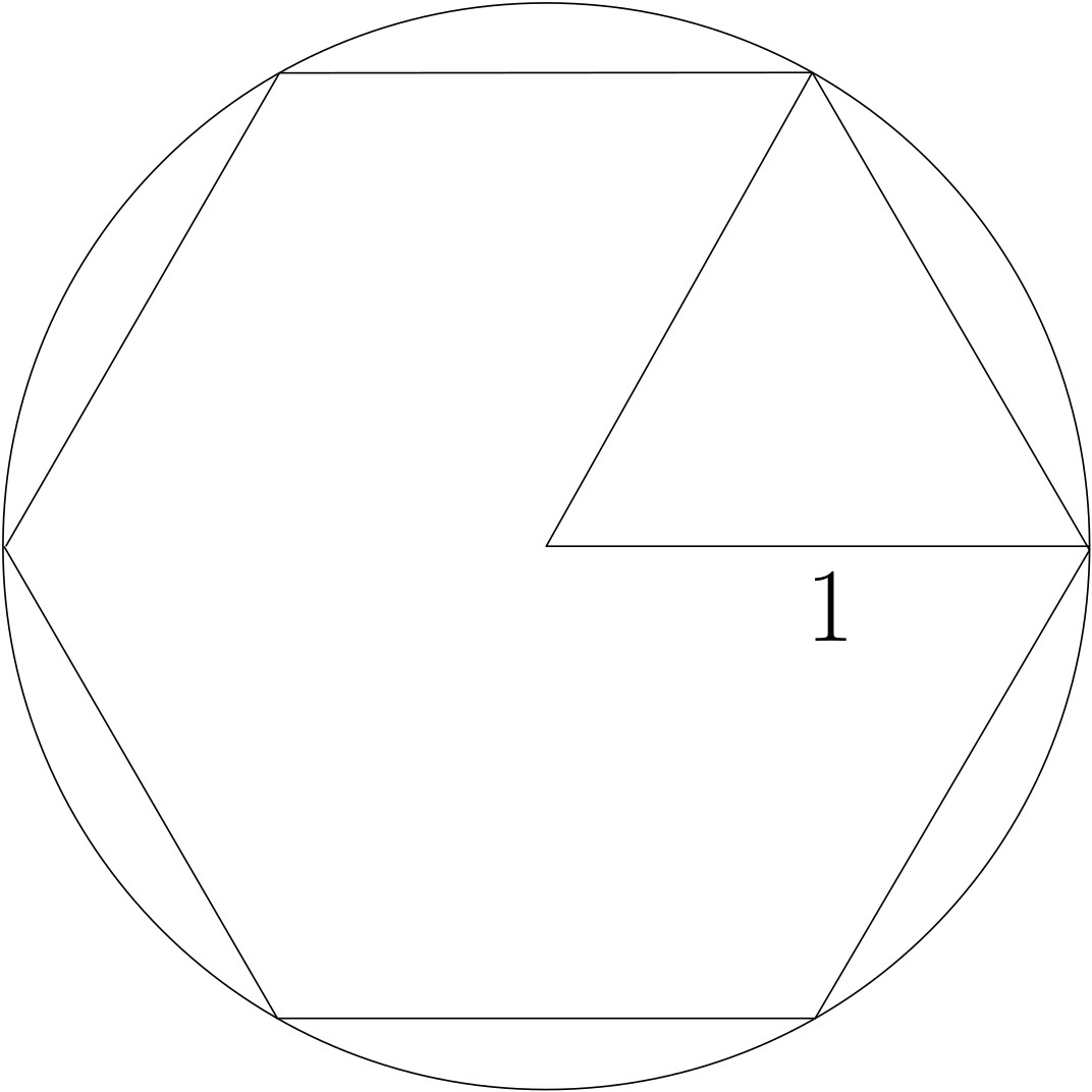
For $n\geq 1$, let $\mathcal{P}_n$ be a regular $3\times 2^n$-gon with radius $1$. Here is $\mathcal{P}_1$:
We will use SymPy to deduce nice formulas for approximations of $\pi$.
## loading python libraries

# necessary to display plots inline:
%matplotlib inline

# load the libraries
import matplotlib.pyplot as plt # 2D plotting library
import numpy as np              # package for scientific computing
from pylab import *

from math import *              # package for mathematics (pi, arctan, sqrt, factorial ...)
import sympy as sympy             # package for symbolic computation
from sympy import *
Symbolic computation is a theory and a set of tools that enable manipulation of exact mathematical expressions without resorting to approximate calculations. In Python, a standard library for symbolic computation is SymPy. The objective of today's tutorial is to learn how to use SymPy to solve various problems typically addressed with pen and paper.
To begin with, run and compare the following scripts:
print('With Numpy: ')
print('root of two is '+str(np.sqrt(2)))
print('the square of (root of two) is '+str(np.sqrt(2)**2))
print('---------')
print('With SymPy: ')
print('root of two is '+str(sympy.sqrt(2)))
print('the square of (root of two) is '+str(sympy.sqrt(2)**2))
With Numpy:
root of two is 1.4142135623730951
the square of (root of two) is 2.0000000000000004
---------
With SymPy:
root of two is sqrt(2)
the square of (root of two) is 2
One can expand or simplify expressions:
print('Simplification/Expansion of algebraic expressions:')
print('the square root of 40 is '+str(sympy.sqrt(40)))
print('(root(3)+root(2))**20 is equal to '+str(expand((sympy.sqrt(3)+sympy.sqrt(2))**20)))
#
print('root(-4) ='+str(sympy.sqrt(-4)))

print('----------------')
print('Simplification of symbolic expressions:')
var('x') # We declare a 'symbolic' variable
Expression=(x**2 - 2*x + 1)/(x-1)
print(str(Expression) + ' simplifies into '+str(simplify(Expression)))
Simplification/Expansion of algebraic expressions:
the square root of 40 is 2*sqrt(10)
(root(3)+root(2))**20 is equal to 4517251249 + 1844160100*sqrt(6)
root(-4) =2*I
----------------
Simplification of symbolic expressions:
(x**2 - 2*x + 1)/(x - 1) simplifies into x - 1
With Sympy one can also obtain Taylor expansions of functions with series:
# Real variable
print('--------------')
print('Taylor expansion for a real variable x')
var('x')
Expression=cos(x)
print('Expansion of cos(x) at x=0: '+str(Expression.series(x,0)))
print('Expansion of cos(x) at x=0 at the order 7: '+str(Expression.series(x,0,8)))

# integer variable
print('--------------')
print('Taylor expansion for a discrete variable n')
var('n',integer=True)
Expression=cos(1/n)
print('Expansion of cos(1/n) when n -> +oo: '+str(Expression.series(n,oo)))   # oo means infinity (!)
--------------
Taylor expansion for a real variable x
Expansion of cos(x) at x=0: 1 - x**2/2 + x**4/24 + O(x**6)
Expansion of cos(x) at x=0 at the order 7: 1 - x**2/2 + x**4/24 - x**6/720 + O(x**8)
--------------
Taylor expansion for a discrete variable n
Expansion of cos(1/n) when n -> +oo: 1/(24*n**4) - 1/(2*n**2) + 1 + O(n**(-6), (n, oo))
SymPy can also compute with "big O's". (By default $O(x)$ is considered for $x\to 0$.)
var('x')

display((x+O(x**3))*(x+x**2+O(x**3)))
print('simplifies into:')
simplify((x+O(x**3))*(x+x**2+O(x**3)))
simplifies into:
var('x y')
formula=simplify((cos(x+y)-sin(x+y))**2)
print(formula)
print(latex(formula))
display(formula)
2*cos(x + y + pi/4)**2
2 \cos^{2}{\left(x + y + \frac{\pi}{4} \right)}
Warning: Fractions such as $1/4$ must be introduced with Rational(1,4) to keep Sympy from evaluating the expression. For example:
print('(1/4)^3 = '+str((1/4)**3))
print('(1/4)^3 = '+str(Rational(1,4)**3))
(1/4)^3 = 0.015625
(1/4)^3 = 1/64
phi=(1+sympy.sqrt(5))/2
formula=(phi**4-phi)/(phi**7+1)
print("F = "+str(formula))
print("simplified F = ")
display(simplify(formula))
F = (-sqrt(5)/2 - 1/2 + (1/2 + sqrt(5)/2)**4)/(1 + (1/2 + sqrt(5)/2)**7)
simplified F =
We will see how to use SymPy to prove a mathematical statement. Our aim is to make as rigorous proofs as possible, as long as we trust SymPy.
def InductionFormula(x,y):
    return (1+x)/y

var('a b')
Sequence=[a,b]

print('u_0 = a')
print('u_1 = b')
for i in range(2,15):
    Sequence.append(simplify(InductionFormula(Sequence[-1],Sequence[-2])))
    print('u_'+str(i)+' = '+str(Sequence[-1]))
u_0 = a
u_1 = b
u_2 = (b + 1)/a
u_3 = (a + b + 1)/(a*b)
u_4 = (a + 1)/b
u_5 = a
u_6 = b
u_7 = (b + 1)/a
u_8 = (a + b + 1)/(a*b)
u_9 = (a + 1)/b
u_10 = a
u_11 = b
u_12 = (b + 1)/a
u_13 = (a + b + 1)/(a*b)
u_14 = (a + 1)/b
Sympy?¶For $n\geq 1$, let $\mathcal{P}_n$ be a regular $3\times 2^n$-gon with radius $1$. Here is $\mathcal{P}_1$:
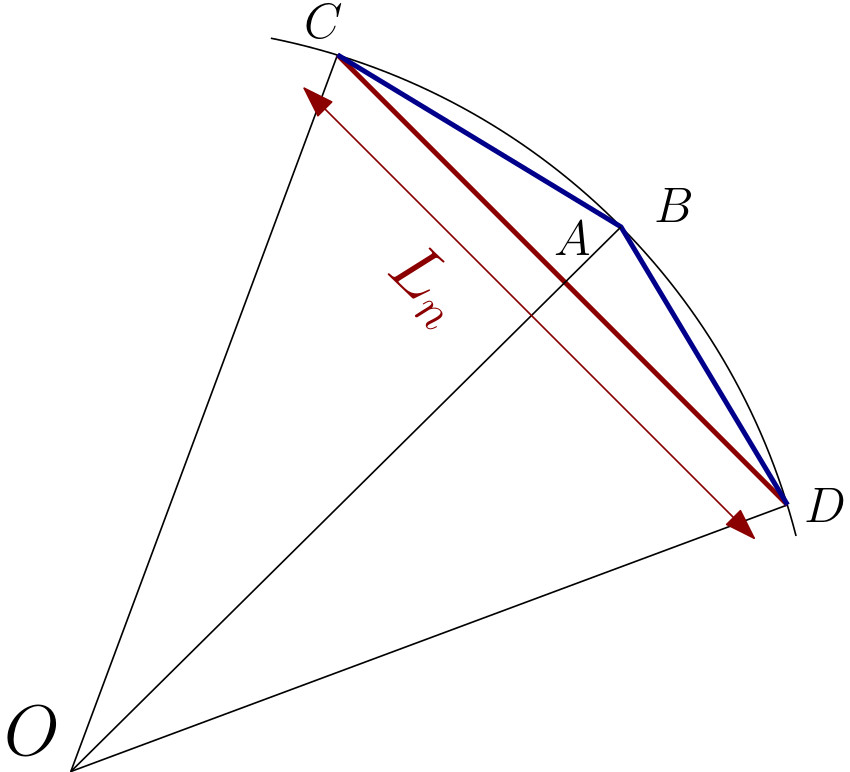
SuccessiveApproximations=[1]
p=11
for n in range(2,p):
    OldValue=SuccessiveApproximations[-1]
    NewValue=sqrt(2-2*sqrt(1-(OldValue**2)*Rational(1,4)))
    SuccessiveApproximations.append(NewValue)
    print('---------------------')
    #display(NewValue)
    print('For n = ',str(n),', i.e. '+str(3*2**n)+' sides, we get 3x2^n L_n =')
    display(simplify(3*(2**(n-1))*NewValue))
    #print(latex(simplify(3*(2**n)*NewValue)))
    print('Numerical value: ',N(NewValue*3*2**(n-1)))
---------------------
For n =  2 , i.e. 12 sides, we get 3x2^n L_n =
Numerical value:  3.10582854123025
---------------------
For n =  3 , i.e. 24 sides, we get 3x2^n L_n =
Numerical value:  3.13262861328124
---------------------
For n =  4 , i.e. 48 sides, we get 3x2^n L_n =
Numerical value:  3.13935020304687
---------------------
For n =  5 , i.e. 96 sides, we get 3x2^n L_n =
Numerical value:  3.14103195089051
---------------------
For n =  6 , i.e. 192 sides, we get 3x2^n L_n =
Numerical value:  3.14145247228546
---------------------
For n =  7 , i.e. 384 sides, we get 3x2^n L_n =
Numerical value:  3.14155760791186
---------------------
For n =  8 , i.e. 768 sides, we get 3x2^n L_n =
Numerical value:  3.14158389214832
---------------------
For n =  9 , i.e. 1536 sides, we get 3x2^n L_n =
Numerical value:  3.14159046322805
---------------------
For n =  10 , i.e. 3072 sides, we get 3x2^n L_n =
Numerical value: 3.14159210599927
One can solve equations with Sympy. The following script shows how to solve $x^2=x+1$:
var('x') # we declare the variable
SetOfSolutions=solve(x**2-x-1,x)
print(SetOfSolutions)
[1/2 - sqrt(5)/2, 1/2 + sqrt(5)/2]
Let $n\geq 1$ be an integer, we are interested in solving the equation \begin{equation} x^3 +nx =1.\tag{$\star$} \end{equation}
In the script below we plot $x \mapsto x^3$, and $x \mapsto 1-nx$ for $0\leq x\leq 1$ and for several (large) values of $n$. This suggests that Equation $(\star)$ has a unique real solution in the interval $[0,1]$, that we will denote by $S_n$.
RangeOf_x=np.arange(0,1,0.01)

plt.plot(RangeOf_x,RangeOf_x**3,label='x $\mapsto$ x^3')

for n in [10, 20, 30]:
    f=[1-n*x for x in RangeOf_x]
    plt.plot(RangeOf_x,f,label='x $\mapsto$ 1-nx for n ='+str(n)+' ')

plt.xlim(0, 1),plt.ylim(-1, 1)
plt.xlabel('Value of x')
plt.legend()
plt.title('Location of S_n')
plt.show()

var('x')
var('n')#,integer=True)

# Question 1.
Solutions=solve(x**3+n*x-1,x)
Sn=Solutions[0]  # The two other solutions are complex numbers
display(Sn)
# Question 2.
Taylor=series(Sn,n,oo,5)
print("Taylor expansion when epsilon -> 0 : "+str(Taylor))
Taylor expansion when epsilon -> 0 : -1/n**4 + 1/n + O(n**(-5), (n, oo))
We consider the following equation: \begin{equation} X^5-3\varepsilon X^4-1=0, \tag{$\star$} \end{equation} where $\varepsilon$ is a positive parameter. As in previous exercise a quick analysis shows that if $\varepsilon>0$ is small enough then ($\star$) has a unique real solution, that we denote by $S_\varepsilon$.
The degree of this equation is too high to be solved by SymPy:
var('x')
var('e')
solve(x**5-3*e*x**4-1,x)
[]
Indeed, SymPy needs help to handle this equation.
In the above script we plotted the function $f(x)=x^5-3\varepsilon x^4-1$ for some small $\varepsilon$. This suggests that $\lim_{\varepsilon \to 0}S_\varepsilon=1$.
RangeOf_x=np.arange(0,2,0.01)

def ToBeZero(x,eps):
    return x**5+x**4*(-3*eps) -1

eps=0.001
plt.plot(RangeOf_x,[ToBeZero(x,eps) for x in RangeOf_x],label='x**5+x**4*(-3*eps)-1')

plt.xlim(0, 2)
plt.ylim(-1, 1)
plt.plot([-2,2],[0,0])
plt.plot([1,1],[-2,2])
plt.xlabel('Value of x')
plt.title('Location of S_eps, with eps ='+str(eps))
plt.legend()
plt.show()

var('r')
var('s')
var('eps')
Expression=ToBeZero(1+r*eps+s*eps**2+O(eps**3),eps)

Simple=simplify(Expression)
print(Simple)

solve([-3+5*r,5*s-12*r+10*r**2],[r,s])
-3*eps + 5*eps*r + 5*eps**2*s - 12*eps**2*r + 10*eps**2*r**2 + O(eps**3)
[(3/5, 18/25)]